Count copies before assigning probabilities
A population can contain many individuals that carry A without having the same proportion of A among its allele copies. An AA individual contributes two copies; an Aa individual contributes one. Counting carriers treats these individuals alike and loses information. The first decision in a population-genetics calculation is therefore what the denominator counts: individuals or copies of a particular locus.
Use a diploid, autosomal locus with only two alleles, A and a, throughout this guide. If there are N individuals, there are 2N copies of that locus. Let p denote the frequency of A and q the frequency of a. Because those are the only alleles in this model, p + q = 1. This accounting identity does not, by itself, demonstrate Hardy-Weinberg equilibrium.
The same allele total can hide different pairings
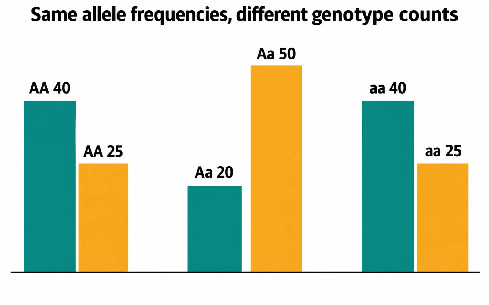
Take an invented sample of 100 individuals: 40 AA, 20 Aa and 40 aa. The A count is (2 x 40) + 20 = 100; the a count is (2 x 40) + 20 = 100. Divide each by 200, not by 100, to obtain p = 0.5 and q = 0.5. Direct counting does not require the sample to be at equilibrium.
Now calculate the Hardy-Weinberg expectations from these allele frequencies: p squared = 0.25, 2pq = 0.50 and q squared = 0.25. For a sample size of 100, those proportions correspond to expected counts of 25 AA, 50 Aa and 25 aa. They are clearly different from the observed 40, 20 and 40, even though both sets contain 100 A copies and 100 a copies.
In the figure, teal bars are the invented observations and amber bars are the model expectations. The discrepancy is in how allele copies are paired into genotypes. Do not overwrite the observations with the calculated bars: prediction and measurement occupy separate columns. This distinction is the main reason to learn the calculation rather than only the formula.
The denominator tells you what you counted
In the 100-individual sample, 60 individuals carry A, but there are 100 A copies among 200 locus copies. The resulting 60% and 50% are both legitimate quantities with different meanings. Write 'individuals carrying A' or 'copies of A' beside the numerator before reaching for p. A percentage without its counted object is incomplete.
Match the evidence to the operation
The model is needed for predicting genotype proportions, not for counting allele copies from known genotypes.
| Available evidence | Valid starting operation | Assumption or limit |
|---|---|---|
| AA, Aa and aa counts | A copies = 2(AA) + Aa; divide by 2N | No equilibrium assumption needed for direct counting |
| p and q under Hardy-Weinberg conditions | Expected genotypes: p squared, 2pq, q squared | These are expectations, not replacement observations |
| Recessive phenotype frequency with equilibrium stated | Identify q squared, then take its positive square root | Requires the stated simple genotype-phenotype relationship |
| Dominant phenotype frequency without equilibrium | Keep AA and Aa unresolved | The phenotype alone does not count A copies |
| Observed counts unlike expected counts | Describe the discrepancy before proposing a cause | Counts alone do not identify selection, drift or mating history |
Where the factor two in 2pq comes from
Under the random-union model, a gamete carrying A can pair with one carrying a, with probability pq. The reverse parental contribution, a followed by A, has probability qp. These are two routes to the same heterozygous genotype, so their probabilities add to 2pq. AA has probability p times p, and aa has probability q times q.
This is a population-level model using allele frequencies in the gamete pools. It is not a statement that every individual is heterozygous or that every mating is Aa x Aa. In the familiar heterozygote cross, each parent's gametes happen to have equal allele probabilities. A population can have those same overall probabilities while containing many different parental genotypes.
The usual equilibrium baseline assumes random mating, enough individuals for drift to be negligible, no selection, no migration and no mutation. Treat these as assumptions to state, not observations proved by the algebra. NCERT Class 12 Biology, Chapter 6, introduces the Hardy-Weinberg principle within Evolution; the supplementary sources explain the distinction between allele counts and genotype expectations.
A recessive phenotype permits an estimate only with assumptions
Suppose an independently constructed exercise states that a fully expressed recessive phenotype occurs in 4% of a population at Hardy-Weinberg equilibrium. Assume one autosomal locus, two alleles, complete dominance, and no ambiguity in phenotype classification. The recessive phenotype identifies aa, so q squared = 0.04 and q = 0.20. It follows that p = 0.80 and the expected heterozygote frequency is 2 x 0.80 x 0.20 = 0.32.
For a population of 2,000 under that idealised model, the expectations are 1,280 AA, 640 Aa and 80 aa. The counts sum to 2,000. A second check counts a copies: 640 from heterozygotes plus 160 from aa gives 800 out of 4,000 copies, or 0.20. This returns the original q and checks that individuals have not been confused with alleles.
The wrong answer q = 0.04 treats a genotype frequency as an allele frequency. A different mistake is calling all 96% with the dominant phenotype AA. That group includes Aa as well. If equilibrium is not supplied or justified, the recessive phenotype alone does not determine how the remaining individuals split between AA and Aa. The missing heterozygote count prevents a unique allele-frequency calculation.
Why a mismatch does not identify its own cause
Return to the observed 40/20/40 sample. It contains fewer heterozygotes than the simple random-union expectation. That observation calls for explanation, but it does not tell us that A is advantageous or that a mutation has occurred. Sampling, population structure, mating patterns and other processes can affect the comparison. Assigning one cause requires evidence beyond the three genotype counts.
Nonrandom mating can change genotype proportions without necessarily changing allele frequencies when other influences are absent. Conversely, observing a set of proportions close to the model at one time does not prove that allele frequencies have remained unchanged across generations. A snapshot of pairing and a time series of allele frequencies answer different questions.
For NEET revision, explain the baseline and recognise the processes that can disturb it. For real data, a small departure from expected counts may simply reflect sampling variation; a formal assessment needs appropriate statistical treatment. The invented chart is not a statistical test, and its purpose is not to infer a real population's mating system.
A dominant allele need not be the common allele
Dominance describes the phenotype of a heterozygote, not an allele's share of the gene pool. Imagine p = 0.10 for A in the equilibrium model. The expected AA frequency is 0.01 and Aa frequency is 0.18, so a completely dominant A phenotype would occur in 0.19 of individuals. A can determine the heterozygote phenotype while remaining the less frequent allele.
There is also a useful boundary check on heterozygosity. With two alleles, 2pq reaches its model maximum of 0.50 when p and q are both 0.50. This is a limit on Hardy-Weinberg expected heterozygosity, not a prohibition against an observed sample containing more than 50% heterozygotes. A deliberately produced group consisting entirely of Aa offspring, for example, is not a random-mating population sample.
Choose the valid starting line without looking at the formula
Write three prompts on paper: genotype counts are known; only a recessive phenotype is known with equilibrium stated; only a dominant phenotype is known without equilibrium stated. For the first, start by counting allele copies. For the second, identify q squared before taking a square root. For the third, explain why the AA/Aa split is unresolved instead of inventing it.
Finally reproduce the 40/20/40 comparison and the 4% example on separate lines. Mark measured counts with O and expected counts with E. Verify that genotype frequencies sum to one and allele copies sum to 2N. End each solution with its assumption: direct counting, or a Hardy-Weinberg prediction. That final label keeps the mathematical result attached to the evidence that supports it.
Common confusions to check
- p + q = 1 alone does not prove equilibrium.
- A recessive phenotype frequency represents q squared only under the stated model.
- Dominant does not mean frequent in the population.
- A genotype-proportion mismatch does not identify an evolutionary cause by itself.
Editorial note and disclaimer
Written by: DongFeng. Published by: MedQGo. Last updated: October 3, 2026.
Disclaimer: This guide is a revision aid for NEET-UG aspirants and does not constitute medical advice. For clinical or health-related queries, consult a qualified medical professional.
References
Related revision guides
How to use this guide
Read the relevant NCERT chapter first. Then redraw the relationships or process described here from memory, compare your version with the textbook, and correct only the gaps. This is an independent revision aid, not official NCERT, NTA, or NEET material.